Excerpt
Index
i
Nanostructure Physics of a Quantum Well adjacent to a tunnel barrier:
analytical calculation and numerical investigations of transcendental equations
obeyed by quasi-bound energy levels
Zuned Ahmed, Md Emrul Hasan and Sujaul Chowdhury
section page number
Chapter
I
Background on Quantum Mechanics
1-
16
1.1 Wave equation of a free particle: Schrödinger equation
2
1.2 Schrödinger equation of a particle subject to a conservative mechanical
force
3
1.3 Allowed values of an observable
5
1.4 Eigenvalue equation, eigenfunction and eigenvalue
6
1.5 Time-independent Schrödinger equation and stationary state.
6
1.6 Continuous and discontinuous function
8
1.7 Finite and infinite discontinuity
10
1.8 Admissibility
conditions on wave function
11
1.9 Calculation of confined energy levels of isolated quantum well (QW)
12
Chapter
II
Background on Microelectronics
17-
33
2.1 Insulator and its band model
18
2.2 Intrinsic semiconductor and its band model
19
2.3 Elemental and compound semiconductors
22
2.4 Alloy semiconductors: ternary and quaternary semiconductors
26
2.5 Bandgap engineering
28
2.6 Substrate and epitaxial layer
31
2.7 Semiconductor heterostructure and heterojunction
31
Index
ii
Chapter
III
Background on Nanostructure Physics
34-
57
3.1.1 Tunnel barrier: structure and band model
35
3.1.2 Transport of electron or hole through tunnel barrier
36
3.2 Quantum
Well
(QW)
41
3.3 Symmetric
double
barrier
47
Chapter
IV
Analytical calculation of transcendental equation
obeyed by quasi-bound energy levels of the Quantum Well
58-
69
4.1 Introduction to the Quantum Well
59
4.2 Analytical calculations of transcendental equations obeyed by quasi-
bound energy levels of the Quantum Well
60
4.3 Recovering results for isolated QW
68
Chapter
V
Analytical calculation of transcendental equation
obeyed by quasi-bound energy levels of the Quantum Well
using another approach
70-
78
5.1 Analytical calculations of transcendental equation obeyed by quasi-
bound energy levels of the Quantum Well: using another approach
71
Chapter
VI
Numerical investigation of
parametric dependence of quasi-bound energy levels of
the Quantum Well
79-
96
6.1 The transcendental equations obeyed by quasi-bound energy levels of
the Quantum Well
80
6.2 The numerical investigation
80
6.3 Conclusions about the parametric variations
96
References 97
Nanostructure Physics of a Quantum Well adjacent to a tunnel barrier: analytical calculation and numerical
investigations of transcendental equations obeyed by quasi-bound energy levels
Zuned Ahmed, Md Emrul Hasan and Sujaul Chowdhury
1
Chapter I
Background on Quantum Mechanics
Chapter I: Background on Quantum Mechanics
2
1.1 Wave equation of a free particle: Schrödinger equation
If we associate the wave packet
)
t
,
x
(
=
2
1
dk
e
)
k
(
a
)
t
kx
(
i
³
+
-
-
where a(k) =
2
1
dx
e
)
t
,
x
(
)
t
kx
(
i
³
+
-
-
-
with a free material particle, we can write
)
t
,
x
(
=
!
2
1
dp
e
)
p
(
a
)
Et
px
(
i
³
+
-
-
!
where a(p) =
!
2
1
dx
e
)
t
,
x
(
)
Et
px
(
i
³
+
-
-
-
!
using de Broglie's equations p =
! k and E =
! . In three dimensions, we have
)
t
,
r
(
&
=
3
)
2
(
1
!
³
-
p
d
e
)
p
(
a
)
Et
r
.
p
(
i
&
&
&
&
!
------------(1.1)
where r
.
p
&
&
=
z
p
y
p
x
p
z
y
x
+
+
. Equation (1.1) gives
x
=
3
x
)
2
(
p
i
!
!
p
d
e
)
p
(
a
)
Et
r
.
p
(
i
&
&
&
&
!
³
-
and
2
2
x
=
3
2
2
x
)
2
(
p
!
!
-
p
d
e
)
p
(
a
)
Et
r
.
p
(
i
&
&
&
&
!
³
-
.
Similarly,
2
2
y
=
3
2
2
y
)
2
(
p
!
!
-
p
d
e
)
p
(
a
)
Et
r
.
p
(
i
&
&
&
&
!
³
-
and
2
2
z
=
3
2
2
z
)
2
(
p
!
!
-
p
d
e
)
p
(
a
)
Et
r
.
p
(
i
&
&
&
&
!
³
-
.
all momentum space
Nanostructure Physics of a Quantum Well adjacent to a tunnel barrier: analytical calculation and numerical
investigations of transcendental equations obeyed by quasi-bound energy levels
Zuned Ahmed, Md Emrul Hasan and Sujaul Chowdhury
3
2
=
3
2
2
z
2
y
2
x
)
2
(
/
)
p
p
p
(
!
!
+
+
-
p
d
e
)
p
(
a
)
Et
r
.
p
(
i
&
&
&
&
!
³
-
=
3
2
2
)
2
(
p
!
!
-
p
d
e
)
p
(
a
)
Et
r
.
p
(
i
&
&
&
&
!
³
-
or,
2
=
2
2
p
!
-
or,
m
2
2
!
-
)
t
,
r
(
2
&
=
m
2
p
2
)
t
,
r
(
&
------------(1.2)
Again, equation (1.1) gives
t
=
!
iE
-
3
)
2
(
1
!
p
d
e
)
p
(
a
)
Et
r
.
p
(
i
&
&
&
&
!
³
-
=
!
iE
-
or, i!
t
= E
-----------(1.3)
For a free particle, E =
m
2
p
2
. Hence equation (1.2) and (1.3) give
m
2
2
!
-
2
= i
!
t
-----------(1.4)
Equation (1.4) is the differential equation for the matter wave of a free particle and
equation (1.4) is called wave equation or Schrödinger equation for a free particle.
Equation (1.4) is a linear equation and hence a monochromatic wave such as
)
Et
r
.
p
(
i
e
)
p
(
a
-
&
&
!
&
as well as a wave packet given by equation (1.1) satisfy it.
1.2 Schrödinger equation of a particle subject to a conservative mechanical
force
1) A comparison of
< x > =
³
x
*
dx
and
< p > =
³
x
i
*
!
dx
shows that expectation value of momentum < p > of a particle having wavefunction
associated with it can be computed in the same way as that of position < x > if the
operator
x
i
!
is substituted in place of x. This statement introduces operator
formalism in quantum mechanics. Thus the operator of x is x, operator of p is
x
i
!
.
Chapter I: Background on Quantum Mechanics
4
By "operator of p is
x
i
!
", we in fact mean, the operator we need to calculate the
expectation value of p is
x
i
!
.
2) The Schrödinger equation of a free particle is
-
2
2
2
x
m
2
!
= i
t
!
.
This equation can be obtained from the classical equation
m
2
p
2
= E by the operator
correspondence of p and E as
x
i
!
and i
t
! respectively, and letting the operators
operate on the wavefunction
. Thus the operator of E is i
t
! .
3) If a conservative force acts on a particle, the total energy E =
m
2
p
2
+ V, where V is
potential energy and hence V is a function of position only. Hence
>
<
)
x
(
V
=
³
+
-
dx
)
t
,
x
(
)
x
(
V
2
=
³
+
-
dx
)
x
(
V
*
Thus the operator of V(x) is V(x).
4) Using the operator correspondences of E, p and V,
m
2
p
2
+ V = E gives
m
2
x
i
2
¸
¹
·
¨
©
§
!
+ V = i
t
! or, -
2
2
2
x
m
2
!
+ V = i
t
!
or,
-
2
2
2
x
m
2
!
+ V
= i
t
!
or,
»
»
¼
º
«
«
¬
ª
+
-
V
x
m
2
2
2
2
!
= i
t
!
.
This is the Schrödinger equation of a particle moving in a potential V. In three
dimensions, [
m
2
2
!
-
2
+ V]
= i
t
!
is the Schrödinger equation of a particle
moving in a potential V. The operator [
m
2
2
!
-
2
+ V] is the operator of total energy
of a conservative system and is called Hamiltonian operator.
Nanostructure Physics of a Quantum Well adjacent to a tunnel barrier: analytical calculation and numerical
investigations of transcendental equations obeyed by quasi-bound energy levels
Zuned Ahmed, Md Emrul Hasan and Sujaul Chowdhury
5
1.3 Allowed values of an observable
Suppose, there exists a state
for which an observable A has an allowed
value of `a' only; and there is no uncertainty. As such,
< A > = a , i.e.
³
d
A
= a and the standard deviation,
A = 0.
or, < (A
- < A >)
2
> = 0
2
)
x
(
=
¦
-
i
2
i
)
x
x
(
n
1
or, <
(A
- a)
2
> = 0 or,
-
³
d
)
a
A
(
2
= 0
< A > =
³
d
A
or,
-
-
³
d
)
a
A
(
)
)
a
A
((
= 0
(A
- a) is Hermitian (proved below)
or,
-
³
d
)
a
A
(
2
= 0
(A - a) = 0
³
d
2
= 0 only if
= 0
or, A
= a
Thus allowed values of an observable are given by the values of `a' that can be
obtained by solving the differential equation A
= a . If one obtains
1
a ,
2
a ,
3
a , ...
as the allowed values, in practice, the allowed values of the observable are in the
ranges a
1
- da
1
to a
1
+ da
1
, a
2
- da
2
to a
2
+ da
2
, a
3
- da
3
to a
3
+ da
3
, ... where d
i
a
is the
uncertainty in
i
a
. There is some uncertainty in every observable quantity, because
there is always some uncertainty in both the position and the momentum of the
associated particle.
We have assumed that (A
- a) is Hermitian. Let us prove it, i.e. let us show
that (
1
, (A - a)
2
) = ((A - a)
1
,
2
).
L.H.S. = (
1
, (A
- a)
2
) =
³
-
d
)
a
A
(
2
*
1
=
³
-
d
)
a
A
(
2
2
*
1
=
³
d
A
2
*
1
-
³
d
a
2
*
1
=
³
d
)
A
(
2
1
-
³
d
)
a
(
2
1
A is observable, A is Hermitian and < A > (= a ) is real
=
³
-
d
]
)
a
(
)
A
[(
2
1
2
1
=
³
-
d
]
)
a
(
)
A
[(
2
1
1
=
³
-
d
)
a
A
(
2
1
1
=
³
-
d
)
)
a
A
((
2
1
= ((A
- a)
1
,
2
) = RHS
(A - a) is Hermitian.
Chapter I: Background on Quantum Mechanics
6
1.4 Eigenvalue equation, eigenfunction and eigenvalue
Allowed values of an observable A are given by solution of the differential
equation A
= a . This equation is called eigenvalue equation, where is called
eigenfunction and a is called eigenvalue. A is operator of the observable.
If we solve the eigenvalue equation A
= a and get the solutions
1
,
2
,
3
, ... and corresponding eigenvalues
1
a ,
2
a ,
3
a , ... respectively, then
i
is
an eigenfunction of the observable A belonging to the eigenvalue
i
a
. The set of all
eigenvalues of an observable is called eigenvalue spectrum.
1.5 Time-independent Schrödinger equation and stationary state.
Schrödinger equation for a particle under conservative force is
-
m
2
2
!
2
)
t
,
r
(
&
+ V
)
t
,
r
(
&
= i
!
t
)
t
,
r
(
&
-----------(1.5)
which is called time-dependent Schrödinger equation. If V(
r
&
) is independent of time,
the Hamiltonian is also time-independent and equation (1.5) simplifies considerably.
Let us try
)
t
,
r
(
&
= u( r
&
) f(t) as a solution of equation (1.5). u is a function of
space coordinates only and f is a function of time t only. Equation (1.5)
-
m
2
2
!
2
[u( r& ) f(t)] + V( r& ) u( r& ) f(t) = i!
t
[u( r
&
) f(t)]
or,
-
m
2
2
!
f(t)
2
u( r& ) + V( r& ) u( r& ) f(t) = i! u( r& )
t
f(t)
or,
-
m
2
2
!
)
r
(
u
)
r
(
u
2
&
&
+ V( r
&
) =
t
)
t
(
f
)
t
(
f
i
!
-----------(1.6)
dividing every term by u( r
&
) f(t)
LHS of equation (1.6) is a function of position only and RHS of equation (1.6) is a
function of time only, because V( r
&
) is a function of position only. Since space
(coordinates) and time are independent (ignoring theory of relativity), equation (1.6)
Nanostructure Physics of a Quantum Well adjacent to a tunnel barrier: analytical calculation and numerical
investigations of transcendental equations obeyed by quasi-bound energy levels
Zuned Ahmed, Md Emrul Hasan and Sujaul Chowdhury
7
makes sense only if both sides of equation (1.6) are equal to a constant, say C. Thus
-
m
2
2
!
)
r
(
u
)
r
(
u
2
&
&
+ V( r
&
)
=
C
-----------(1.7)
and
t
)
t
(
f
)
t
(
f
i
!
=
C
-----------(1.8)
Equation (1.7)
-
m
2
2
!
2
u( r& ) + V( r& ) u( r& ) = C u( r& )
or, [
-
m
2
2
!
2
+ V( r& )] u( r& ) = C u( r& )
----------(1.9a)
or,
op
H
u( r
&
) = C u( r
&
)
----------(1.9b)
op
H
is Hamiltonian operator, i.e. operator of total energy. Equation (1.9) is
eigenvalue equation of total energy.
C is an eigenvalue of total energy (an
observable).
C is real. Let us denote C by E. Equation (1.9)
[
-
m
2
2
!
2
+ V( r& )] u( r& ) = E u( r& )
--------(1.10a)
or,
op
H
u( r
&
) = E u( r
&
)
--------(1.10b)
Equation (1.10) is called time-independent Schrödinger equation.
Equation (1.8)
i
!
t
f(t) = E f(t) or,
dt
d
f(t) =
)
t
(
f
i
E
!
Let, f(t) =
nt
e
nt
ne
= E
!
i
1
nt
e
or, (n
- E
!
i
1
)
nt
e
= 0
n - E
!
i
1
= 0
nt
e
0
or, n = E
!
i
1
=
-
!
iE
=
- i
f(t) =
t
i
e
-
=
Et
i
e
!
-
( r& , t) = u( r& ) f(t) = u( r& )
Et
i
e
!
-
= u( r
&
)
t
i
e
-
----------(1.11)
2
)
t
,
r
(
&
=
*
( r& , t) ( r& , t) = u*( r& )
t
E
i
*
e
!
u( r
&
)
Et
i
e
!
-
= u*( r
&
) u( r
&
)
E is real,
E* = E.
=
2
)
r
(
u
&
---------(1.12)
Chapter I: Background on Quantum Mechanics
8
From equation (1.12), we find that
2
)
t
,
r
(
&
is independent of time. Thus the states
given by equation (1.11) are stationary states.
Expectation value of any observable A is
< A > =
³
d
)
t
,
r
(
A
)
t
,
r
(
op
*
&
&
=
³
-
d
]
e
)
r
(
u
[
A
e
)
r
(
u
Et
i
op
t
E
i
*
*
!
!
&
&
using eqn (1.11)
=
³
-
d
)
r
(
u
A
e
e
)
r
(
u
op
Et
i
Et
i
*
&
&
!
!
E is real
If
op
A
does not explicitly contain the variable t (time)
=
³
d
)
r
(
u
A
)
r
(
u
op
*
&
&
For stationary states, expectation value of any observable A is independent of time,
provided the operator
op
A
itself does not depend explicitly on t.
In hydrogen atom, e.g., the potential V(r) =
0
4
1
-
r
e
is a function of position
only. Thus the solutions of equation (1.5) will give stationary states. Thus
2
for
the electron and the expectation value of all observables (e.g. energy) of the electron
remains independent of time. This explains why hydrogen atom is stable; thus we get
an explanation of one of the ad hoc assumptions of Bohr that the electron in
hydrogen atom stays in stationary state.
1.6 Continuous and discontinuous function
x
f(x)
O
Nanostructure Physics of a Quantum Well adjacent to a tunnel barrier: analytical calculation and numerical
investigations of transcendental equations obeyed by quasi-bound energy levels
Zuned Ahmed, Md Emrul Hasan and Sujaul Chowdhury
9
f(x) above is a continuous function. It is single-valued at every value of x.
dx
df
is also
continuous and single-valued.
f(x) above is a discontinuous function of x. The discontinuity is at x = x
0
where the
function is many valued. f(x
0
) is unspecified. f
1
< f(x
0
) <
2
f .
0
Lt
f(x
0
-
) =
2
f
0
Lt
f(x
0
+
) =
1
f .
dx
df
at x = x
0
- is tan
1
,
dx
df
at x = x
0
+
is tan
2
. Here 0.
x
f(x)
O
x
0
1
2
x
f(x)
O
f
1
f
2
x
0
Chapter I: Background on Quantum Mechanics
10
1
and
2
may or may not be equal, depending on the nature of f(x). Thus the
derivative
dx
df
may or may not be continuous. At x =x
0
,
dx
df
= tan 90
° =
.
1.7 Finite and infinite discontinuity
The discontinuity considered above is finite discontinuity, because
1
f
and
2
f
are finite. If a < f(x
0
) < b where either a or b (or both) is +
or
-
, the discontinuity
is infinite discontinuity.
0
Lt
f(x
0
+
) = a,
0
Lt
f(x
0
- ) = + , a < f(x
0
) <
.
x
f(x)
O
90
°
x
0
x
f(x)
O
x
0
a
Nanostructure Physics of a Quantum Well adjacent to a tunnel barrier: analytical calculation and numerical
investigations of transcendental equations obeyed by quasi-bound energy levels
Zuned Ahmed, Md Emrul Hasan and Sujaul Chowdhury
11
1.8 Admissibility conditions on wave function
1.
(x , t)
0 as x
± , because
³
dx
2
= 1 is finite.
2.
(x, t) must be finite, single-valued and continuous function of x for all time t;
this is because of probability interpretation of
.
3.
t
is a continuous function of x, because otherwise
t
= c where
1
c
< c <
2
c
at
say x = x
0
.
This means
= c t which is many-valued at x = x
0
. But
must be single-valued,
according to condition (2).
4.
x
must be continuous function of x if V(x , t) is continuous. Because, if V(x, t)
is continuous, V(x, t)
(x, t) is continuous.
t
is also continuous (condition (3))
function of x. Hence Schrödinger equation i
!
t
t)
(x,
=
-
m
2
2
!
2
2
x
(x , t) +V(x , t)
(x , t) gives
2
2
x
is continuous. Thus
x
is continuous function of x; otherwise
2
2
x
becomes infinite at points (x) where
x
is discontinuous.
x
t
O
c
1
c
2
x
0
all space
Chapter I: Background on Quantum Mechanics
12
5.
x
must be continuous function of x if V does not have infinite discontinuity. In
Schrödinger equation i
!
t
=
-
m
2
2
!
2
2
x
+ V(x, t) (x, t),
t
is always
continuous function of x (condition 3). If
x
has any discontinuity say at x = x
0
, the
x
versus x curve becomes vertical at x = x
0
and hence its slope
2
2
x
becomes
infinite at x = x
0
. Thus
-
m
2
2
!
2
2
x
=
-
. This forces V to become + to keep the
Schrödinger equation valid. Since
is finite, continuous and single valued
everywhere, V is forced to be +
at x = x
0
. Thus unless V has an infinite
discontinuity,
x
must be a continuous function of x.
Any finite discontinuity of V makes V
finite discontinuous. This is adjusted
by a finite discontinuity of
2
2
x
because
t
is always continuous (see Schrödinger
equation). Finite discontinuity of
2
2
x
means
x
is continuous, otherwise
2
2
x
gets infinite discontinuity there.
1.9 Calculation of confined energy levels of isolated quantum well (QW)
x
V(x)
Region I
- b/2
+ b/2
V
0
V
0
Region II
Region III
(0, 0)
Nanostructure Physics of a Quantum Well adjacent to a tunnel barrier: analytical calculation and numerical
investigations of transcendental equations obeyed by quasi-bound energy levels
Zuned Ahmed, Md Emrul Hasan and Sujaul Chowdhury
13
Figure shows isolated quantum well (QW) of width b and depth V
0
.
V(x) = 0
for b/2 < x < +b/2
V(x) =
0
V for
x > b/2
Let us consider a particle of total energy E <
0
V in the well. We wish to find
allowed values of the total energy E of the particle for motion only along x direction
in the well. By the choice of origin, potential energy is zero inside the QW and hence
E is kinetic energy of the particle for motion only along x direction in the QW.
For region II,
2
2
2
dx
u
d
+
2
m
2
!
(E
- 0)
2
u = 0 or,
2
2
2
dx
u
d
+
2
2
u = 0,
2
=
2
mE
2
!
2
u (x) = A cos
x + B sin x,
2
(x, t) =
2
u (x)
t
E
i
e
!
-
For region I and III,
2
2
dx
u
d
+
2
m
2
!
(E
-
0
V )u = 0
or,
2
2
dx
u
d
-
2
m
2
!
(
0
V
- E)u = 0 since E < V
0
or,
2
2
dx
u
d
-
2
u = 0, where
2
=
2
m
2
!
(
0
V
- E)
u(x) = C
x
e
+ D
x
e
-
.
For region I, we take D = 0; otherwise D
x
e
-
as x- .
1
u (x)= C
x
e
for x <
- b/2,
1
(x, t) =
1
u (x)
t
E
i
e
!
-
For region III, we take C = 0; otherwise C
x
e
as x
+
3
u (x) = D
x
e
-
for x > b/2,
3
(x, t) =
3
u (x)
t
E
i
e
!
-
At x = + b/2,
2
u
(x = + b/2
-
) =
3
u (x = + b/2
+
)
or, A cos
b/2 + B sin
b/2 = D
b/2
e
-
---------(1.13)
At x = + b/2,
-
+
= b/2
x
2
dx
du
=
+
+
=
2
/
b
x
3
dx
du
Chapter I: Background on Quantum Mechanics
14
or,
-
A sin
b/2 +
B cos
b/2 =
- D
b/2
e
-
---------(1.14)
At x =
- b/2,
2
u
(x =
-
+
b/2 ) =
1
u (x =
-
-
b/2 )
or, A cos
b/2
- B sin
b/2 = C
2
/
b
e
-
----------(1.15)
At x =
- b/2,
+
-
=
2
/
b
x
2
dx
du
=
-
-
=
2
/
b
x
1
dx
du
or,
A sin
b/2 +
B cos
b/2 =
C
2
/
b
e
-
---------(1.16)
Eqn (1.13) + (1.15)
2A
cos
b/2 = (C + D)
2
/
b
e
-
---------(1.17)
Eqn (1.13) (1.15)
2B
sin
b/2 = (D
- C)
2
/
b
e
-
---------(1.18)
Eqn (1.14) + (1.16)
2
B cos
b/2 =
(C - D)
2
/
b
e
-
---------(1.19)
Eqn (1.16) (1.14)
2
A sin
b/2 =
(C + D)
2
/
b
e
-
---------(1.20)
Eqn (1.20) / eqn (1.17)
tan
b/2 =
---------(1.21)
Eqn (1.19) / eqn (1.18)
cot
b/2 =
-
---------(1.22)
Eqn (1.21)
tan(
b/2) =
/
---------(1.23)
or,
2
2
0
2
mE
2
)
E
V
(
m
2
mE
2
2
b
tan
!
!
!
-
=
¸¸¹
·
¨¨©
§
or,
1
E
V
mE
2
2
b
tan
0
2
-
=
¸¸¹
·
¨¨©
§
!
---------(1.24)
Equation (1.22)
cot(
b/2) =
- /
---------(1.25)
or,
2
2
0
2
mE
2
)
E
V
(
m
2
mE
2
2
b
cot
!
!
!
-
=
¸¸¹
·
¨¨©
§
-
or,
1
E
V
mE
2
2
b
cot
0
2
-
=
¸¸¹
·
¨¨©
§
-
!
-------(1.26)
Equation (1.24) and (1.26) are trancendental equations obeyed by allowed values of
total energy E of a particle for motion only along x direction inside the isolated QW.
Let
p
=
¸¸¹
·
¨¨©
§
2
mE
2
2
b
tan
!
----------(1.27)
q =
¸¸¹
·
¨¨©
§
-
2
mE
2
2
b
cot
!
----------(1.28)
Nanostructure Physics of a Quantum Well adjacent to a tunnel barrier: analytical calculation and numerical
investigations of transcendental equations obeyed by quasi-bound energy levels
Zuned Ahmed, Md Emrul Hasan and Sujaul Chowdhury
15
and
r =
1
E
V
0
- ---------(1.29)
We can plot p, q and r as functions for E and obtain plots like:
0
50
100
150
200
0
2
4
6
8
10
0
50
100
150
200
0
2
4
6
8
10
E
+
meV
/
po
r
q
or
r
Figure showing p, q and r as functions of E. (see equation (1.27), (1.28) and
(1.29)). Here p, q and r are given by thin curve, thick curve and dashed curve
respectively. The values of E for which the dashed curve intersects with the other
curves satisfy equation (1.24) and (1.26) and hence are allowed values of E of a
particle for motion only along x direction in the quantum well. It may be noted that,
since the dashed curve meets the E axis at non-zero value of E and the thin curve
starts at E = 0, there is always at least one point of intersection for any possible
values of quantum well width and depth. Detailed calculation of allowed values of E
can be found in ISBN: 978-3838377469.
We now obtain another form for equation (1.23) in the following.
)
2
/
b
(
tan
1
)
2
/
b
tan(
2
)
2
/
b
(
sin
)
2
/
b
(
cos
)
2
/
b
cos(
)
2
/
b
sin(
2
b
cos
b
sin
b
tan
2
2
2
-
=
-
=
=
¸
¹
·
¨
©
§
-
-
-
=
1
E
V
1
1
E
V
2
0
0
using equation (1.24)
Chapter I: Background on Quantum Mechanics
16
or,
b
tan
(
)
E
V
E
)
E
V
(
E
2
0
0
-
-
-
=
or,
0
0
2
V
E
2
)
E
V
(
E
2
b
mE
2
tan
-
-
=
¸
¸
¹
·
¨
¨
©
§
!
---------(1.30)
Equation (1.30) is an alternative form of equation (1.24). Equation (1.30) is a
trancendental equation obeyed by allowed values of total energy E of a particle for
motion only along x direction inside the QW.
We now obtain another form for equation (1.25) in the following.
1
)
2
/
b
(
cot
)
2
/
b
cot(
2
)
2
/
b
(
sin
)
2
/
b
(
cos
)
2
/
b
cos(
)
2
/
b
sin(
2
b
cos
b
sin
b
tan
2
2
2
-
=
-
=
=
1
1
E
V
1
E
V
2
0
0
-
¸
¹
·
¨
©
§
-
-
-
=
using equation (1.26)
or, b
tan
(
)
E
V
E
)
E
V
(
E
2
0
0
-
-
-
=
or,
0
0
2
V
E
2
)
E
V
(
E
2
b
mE
2
tan
-
-
=
¸
¸
¹
·
¨
¨
©
§
!
---------(1.31)
Equation (1.31) is an alternative form of equation (1.26). Equation (1.31) is a
trancendental equation obeyed by allowed values of total energy E of a particle for
motion only along x direction inside the QW.
Nanostructure Physics of a Quantum Well adjacent to a tunnel barrier: analytical calculation and numerical
investigations of transcendental equations obeyed by quasi-bound energy levels
Zuned Ahmed, Md Emrul Hasan and Sujaul Chowdhury
17
Chapter II
Background on Microelectronics
Chapter II Background on Microelectronics
18
2.1 Insulator and its band model
A number of allowed energy bands are completely filled and above these
bands, there is a series of completely empty bands at 0 K. Between the highest filled
band called valence band (VB) and the next empty band called conduction band
(CB), the energy gap is large, of the order of 5 to 10 eV. As such it is not possible at
practical temperatures to thermally excite and thereby take an appreciable number of
electrons across the gap from near the top of VB (E
v
) to near the bottom of CB (E
c
).
As such all the energy bands are either completely filled or completely empty at any
practical temperature.
If we apply an external electric field, there is no electron in CB to participate
in electrical conduction. Electrons of completely filled VB cannot find any empty
and allowed state nearby in energy to go to if their kinetic energy would increase by
being accelerated by the electric field; hence electrons of VB cannot participate in
electrical conduction. As such no observable electrical current is caused by applied
electric field. All solids having such energy band model and such electrical
conductivity are classified as insulator, example: diamond having band gap of 7 eV.
Figure 2.1: Band model of insulator (at 0 K). The energy gap E
g
is large and energy
bands are narrow.
Fermi energy for insulator at 0 K is given by
E
F
=
2
v
E
c
E
+
------------(2.1)
CB
VB
Higher
energy of
electron
E
c
E
F
E
v
E
F
=
2
v
E
c
E
+
E
g
Meaningless
Excerpt out of 99 pages
- Quote paper
- Dr Sujaul Chowdhury (Author)Zuned Ahmed (Author)Emrul Hasan (Author), 2014, Nanostructure Physics of a Quantum Well adjacent to a tunnel barrier, Munich, GRIN Verlag, https://www.grin.com/document/273772
Similar texts


Publish now - it's free
✕
Excerpt from
99
pages

Comments