General Relativistic Static Fluid Solutions with Cosmological Constant

Page 3

1 Introduction

This diploma thesis analyses static, spherically symmetric perfect fluid solutions to Einstein’s field equations with cosmological constant. New kinds of global solutions are described.

By a global solution one means an inextendible spacetime satisfying the Einstein equations with cosmological constant with a perfect fluid source. The matter either occupies the whole space or has finite extend. In the second case a vacuum solution is joined on as an exterior field. Global static fluid ball solutions with finite radius at which the pressure vanishes are called stellar models.

Recent cosmological observations give strong indications for the presence of a positive cosmological constant with Λ < 3 × 10 ⁻⁵² m ⁻² . On the other hand Anti-de Sitter spacetimes, having negative cosmological constant, are important in the low energy limit of superstring theory. Therefore it is interesting to analyse solutions to the field equations with cosmological constant representing for example relativistic stars.

Vanishing cosmological constant Λ = 0

The first static, spherically symmetric perfect fluid solution with constant density was already found by Schwarzschild in 1918. In spherical symmetry Tolman [24] and Oppenheimer and Volkoff [17] reduced the field equations to the well known TOV equation. The boundary of stellar models is defined to be where the pressure vanishes. At this surface a vacuum solution is joined on as an exterior field. In case of vanishing cosmological constant it is the Schwarzschild solution. For very simple equations of state Tolman integrated the TOV equation and discussed solutions. Although he already included the cosmological constant in his calculations he did not analyse them. He stated that the cosmological constant is too small to produce effects.

Buchdahl [2] assumed the existence of a global static solution, to show that the total mass of a fluid ball is bounded by its radius. He showed the strict inequality M < (4/9)R, which holds for fluid balls in which the density does not increase outwards. It implies that radii of fluid balls are always larger than the black-hole event horizon. Geometrical properties of constant density solutions were analysed by Stephani [20, 21]. He showed that they can be embedded in a five dimensional flat space and that they are conformally flat. The cosmological constant can easily be included in his calculations by redefining some variables.

Page 7

2 Cosmological TOV equation

This chapter deals with the Einstein field equations with cosmological constant in the spherically symmetric and static case. For a generalised Birkhoff theorem see [22, 19].

First a perfect fluid is assumed to be the matter source. This directly leads to a Λ-extended Tolman-Oppenheimer-Volkoff equation which will be called TOV-Λ equation. The TOV-Λ equation together with the mean density equation form a system of differential equations. It can easily be integrated if a constant density is assumed.

Next a vacuum solution, namely the Schwarzschild-de Sitter solution, is derived. It is the unique static, spherically symmetric vacuum solution to the field equations with cosmological constant with group orbits having non-constant volume. But there is one other static, spherically symmetric vacuum solution, the Nariai solution [15, 16]. The group orbits of this solution have constant volume. The Nariai solution is needed to join interior and exterior solution in a special case but will not be derived explicitly. Finally in this introductory chapter Newtonian limits are derived. Limits of the Schwarzschild-de Sitter solution and the TOV-Λ equation are shown. The second leads to the fundamental equation of Newtonian astrophysics with cosmological constant.

2.1 The Cosmological Constant

Originally the Einstein field equations read

G µν = κT µν , (2.1)

where κ is the coupling constant. Later Einstein [7] introduced the cosmological constant mainly to get a static cosmological solution. These field equations are

G µν + Λg µν = κT µν . (2.2)

The effect of Λ can be seen as a special type of an energy-momentum tensor. It acts as an unusual fluid

with P ^Λ = −Λ/κ and equation of state P ^Λ = −ρ ^Λ c ² .

Page 8

2.2 Remarks on the Newtonian limit

The metric for a static, spherically symmetric spacetime can be written

ds ² = −c ² e ^ν(r) dt ² + e ^a(r) dr ² + r ² (dθ ² + sin ² θ dφ ² ). (2.3)

Appendix B of [11] shows that r ² in front of the sphere metric is no loss of generality for a perfect fluid. This is true for vanishing cosmological constant. With cosmological term there is one vacuum solution with group orbits of constant volume, the mentioned Nariai solution [15, 16]. Metric (2.3) contains the constant c representing the speed of light. Define λ = 1/c ² , roughly speaking the limit λ → 0 corresponds to the Newtonian theory. But equations could be non-regular in the limit λ = 0. Therefore, following [4, 5, 6], the static, spherically symmetric metric has to be written

1 ds ² = − e ^λν(r) dt ² + e ^a(r) dr ² + r ² dΩ ² , (2.4) λ

with field equations

G µν + λΛg µν = κT µν , (2.5)

where dΩ ² = dθ ² + sin ² θ dφ ² . The new term λν(r) in (2.4) ensures regularity of the energy-momentum conservation in the limit if matter is present. The λΛ term in the field equations (2.5) makes sure that the gravitational potential is regular in the limit λ = 0.

2.3 TOV-Λ equation

Assume a perfect fluid to be the source of the gravitational field. The derivation of the analogous Tolman-Oppenheimer-Volkoff [17, 24] equation is shown. Consider metric (2.4)

1 ds ² = − e ^λν(r) dt ² + e ^a(r) dr ² + r ² dΩ ² . λ

Units where G = 1 will be used, thus κ = 8πλ ² . λ = 1 corresponds to Einstein’s theory of gravitation in geometrised units. The field equations (2.5) for a perfect fluid can be taken from appendix A, (A.4)-(A.7) with (A.9). These are three independent equations, which imply energy-momentum conservation (A.10). Thus one may either use three independent field equations or one uses two field equations and the energymomentum conservation equation. The aim of this section is to derive a

Page 11

In addition it should be remarked how w eff is given,

The possibility of writing the equations with effective values is of interest later.

2.4 Schwarzschild-anti-de Sitter and Schwarzschild-de Sitter solution

A vacuum solution (T µν = 0) to the Einstein field equations with cosmological constant is derived. For a vanishing cosmological constant the Schwarzschild solution follows, for vanishing mass the metric gives the de Sitter cosmology. Again one uses metric (2.4)

One has to find a solution to the system of equations

G µν + λΛg µν = 0.

In the static, spherically symmetric case this system reduces to three equations. But there are only two unknown functions. The third equation is not independent. Thus it suffices to consider the first two field equations (A.4),(A.5), given in appendix A.

The first equation gives

and can be integrated to

where 2M is a constant of integration. The additional λ in front of the constant of integration is to get interior (2.14) and exterior metric continuous at a boundary.

Page 13

2.5 Newtonian limits

The Newtonian limits of the Schwarzschild-anti-de Sitter and Schwarzschildde Sitter metric and of the TOV-Λ equation are derived. The frame theory approach by Ehlers [4, 5, 6] will be used to define a one-parameter family of general relativistic spacetime models with Newtonian limit. Including the cosmological term gives a Newtonian limit with a Λ-corrected gravitational potential.

2.5.1 Limit of Schwarzschild-anti-de Sitter and Schwarzschild-de Sitter models

A parametrisation of the Schwarzschild-de Sitter metric is given by (2.22)

ds ² = −

−λg αβ (λ), g ^αβ (λ), Γ ^γ In the limit λ = 0 the family M(λ) = αβ (λ) converges

to a field of a mass point at the origin. The black-hole event horizon and the cosmological event horizon both shrink to a point. The gravitational field is given by

all others vanish. This corresponds to Newton’s equation with cosmological term

2.5.2 Limit of the TOV-Λ equation

The parametrised metric (2.14) is given by

The parametrisation of the TOV-Λ equation (2.16) is

Page 15

3 Solutions with constant density

For practical reasons the notation is changed to geometrised units where c ² = 1/λ = 1.

Assume a positive constant density distribution ρ = ρ 0 = const. Then w = 4π 3 ρ 0 gives (2.16) in the form

In the following all solutions to the above differential equation are derived, see [20, 23, 24]. In [20, 24] the equation was integrated but not discussed for the different possible values of Λ. In [23] all cases with Λ < 4πρ ⁰ were discussed using dimensionless variables. This complicated the physical interpretation of the results and was an unnecessary restriction to the cosmological constant.

The central pressure P c = P (r = 0) is always assumed to be positive and finite. Using that the density is constant in (2.17) metric (2.14) reads

P c + ρ 0

ds ² = − dt ² + r 2 + r ² dΩ ² . (3.2) 8π 3 ρ 0 + Λ P (r) + ρ 0 1 − 3

The metric is well defined for radial coordinates r ∈ [0, ˆ r) if Λ > −8πρ 0 ,

r denotes the zero of g ^rr . If Λ ≤ −8πρ 0 the metric is well defined for where ˆ all r.

Solutions of differential equation (3.1) are uniquely determined by the three parameters ρ 0 , P c and Λ. Therefore one has a 3-parameter family of solutions.

The two cases of negative and positive cosmological constant are discussed separately. In the first case there is no cosmological event horizon whereas in the second there is. Analogous Buchdahl [2] inequalities (3.38) will be derived for the different cases.

Figures of the pressure are shown. The constant density ρ 0 and the central pressure P c are equal in all figures, ρ 0 = P c = 1. Only the cosmological constant varies. This follows the approach of the chapter and helps to compare the different functions.

The end of the chapter summarises the different solutions. An overview is given.

Page 16

3.1 Spatial geometry of solutions

Before starting to solve the TOV-Λ equation one should have a closer look at metric (3.2).

The aim of this section is to describe the spatial geometry of metric (3.2) because it depends on the choice of the constant density ρ 0 and the cosmological constant Λ. For vanishing cosmological constant this was done in [21].

For spherically symmetric spacetimes there exists an invariantly defined mass function [28], the quasilocal mass. For metric (3.2) quasilocal mass [28] is given by

If R denotes the boundary of a stellar object then

where M denotes the total mass of the object. Let

then the the spatial part of metric (3.2) reads

and the quasilocal mass (3.3) is given by

2m q (r) = kr ³ , (3.5)

For all positive values of k spatial metric (3.4) describes one half of a √ 3-sphere of radius 1/ k. The quasilocal mass m q (r) is positive. Introducing a new coordinate by

gives

Page 17

This shows that (3.2) has a coordinate singularity. The metric with radial coordinate r only describes one half of the 3-sphere. Geometrically the coordinate singularity is easily explained. The volume of group orbits r = const. √

has an extremum at the equator ˆ r = 1/ k. Thus this coordinate cannot be used to describe the second half of the 3-sphere. √

Differential equation (3.1) is singular at ˆ r = 1/ k. With the new

coordinate α the differential equation is regular at the the corresponding α(ˆ r) = π/2.

If k = 0 then m q (r) = 0 and the spatial metric is purely Euclidean in spherical coordinates. In Cartesian coordinates this simply reads

dσ ² = dx ² + dy ² + dz ² .

Finally, negative values of k in the spacial metric correspond to threedimensional hyperboloids with negative quasilocal mass. Then using

gives

The coordinate singularity becomes important if Λ exceeds an upper limit. The restriction to Λ < 4πρ 0 in [23] is due to this fact. Up to this limit the radial coordinate r and the new coordinate α are used side by side. Although the radial coordinate is less elegant the physical picture is clearer. In appendix B it will be shown that constant density solutions are con-formally flat [20]. Conformally flat constant density solutions were analysed in [22] and were called generalised solutions of the interior Schwarzschild solution.

If the density is decreasing or increasing outwards solutions are not con-formally flat.

It will also be seen that models with a real geometric singularity exists. They are physically not relevant because the pressure is divergent at the singularity.

3.2 Solutions with negative cosmological constant

In the Schwarzschild-anti-de Sitter spacetime there exists a black-hole event horizon. It will be shown that radii of stellar objects are always larger than this radius corresponding to the black-hole event horizon.

Page 18

3.2.1 Stellar models with spatially hyperbolic geometry

Λ < −8πρ 0

If Λ < −8πρ 0 then k and m q (r) are negative. With (3.7) the denominator of (3.1) can be written as (cosh ² α) and the differential equation does not have a singularity.

The volume of group orbits has no extrema, thus metric (3.2) has no coordinate singularities and is well defined for all r. Write the differential equation (3.1) as

Integration gives

C is the constant of integration, evaluated by defining P (α = 0) = P c to be the central pressure. At the centre it is found that

Throughout this calculation it is assumed that 8πρ 0 < −Λ. With P c > 0 this implies that C > 3 and (1 − Λ/4πρ 0 ) > 3, which can easily be verified. The constant C will be used instead of its explicit expression given by (3.10). Then the pressure reads

The function P (α) is well defined and monotonically decreasing for all α. The pressure converges to −ρ 0 as α or as the radius r tends to infinity. Thus a radius R, where the pressure vanishes, always exists. It is given by

Writing it in α, where α b corresponds to R

Page 20

Figure 1: Pressure function P (α) with ρ 0 = 1, P c = 1 and Λ = −10π

Figure 2: Radius as a function of

central pressure R = R(P c )

this and many of the following cases. Therefore the next section shows this procedure explicitly.

Figure 1 shows the typical behaviour of function P (α) (3.11). Figures 2 and 3 show the radius of the object as a function of the central pressure (3.12) and the radius as a function of the new variable α (3.7), respectively. Constant density and central pressure are both set to one, ρ 0 = 1, P c = 1.

3.2.2 Joining interior and exterior solution

At the P = 0 surface the Schwarzschild-anti-de Sitter solution (2.22) is joined. Since this is needed for all solutions describing stellar objects the procedure of joining interior and exterior solution is shown explicitly. Gauss coordinates to the r = const. hypersurfaces in the interior are

Page 22

where P ^′ (χ b ) can be derived from (3.1) to give √

With (3.20) both equations combine to

√

For the exterior metric one finds

Use (3.19) for the first term and (3.20) for the last term. Furthermore the mass is given by √

see (2.10). Then this derivative evaluated at χ b reads

√

which equals equation (3.21). Thus the metric is C ¹ at χ b . Since the density is not continuous at the boundary the Ricci tensor is not, either. Therefore the metric is at most C ¹ . This cannot be improved.

3.2.3 Stellar models with spatially Euclidean geometry

Λ = −8πρ 0

Assume that cosmological constant and constant density are chosen such that 8πρ 0 = −Λ. Then k = 0, m q (r) = 0 and the denominator of (3.1) becomes one. The differential equation simplifies to

dP

= −4πr (P + ρ 0 ) ² , (3.23) dr

and the t = const. hypersurfaces of (3.2) are purely Euclidean. As in the former case metric (3.2) is well defined for all r.

Page 24

Figure 4: Pressure function P (r) with ρ 0 = 1, P c = 1 and Λ = −8π

3.2.4 Stellar models with spatially spherical geometry

Λ > −8πρ 0

If Λ > −8πρ 0 then k and m q (r) are positive. Equation (3.1) has a singularity at

In α the singularity ˆ r corresponds to α(ˆ r) = π/2.

As already mentioned in section 3.1 the spatial part of metric (3.2) now √

describes part of a 3-sphere of radius 1/ k. The metric is well defined for radii less than ˆ r. Integration of (3.1) gives

One finds

which is less than zero if Λ < 4πρ 0 , which is the restriction in [23]. Since this is the considered case the singularity of the pressure gradient is not important yet.

C is a constant of integration and can be expressed by the central pressure P c . Again one obtains

Page 27

3.3 Solutions with vanishing cosmological constant

Assume a vanishing cosmological constant. Then one can use all equations of the former case with Λ = 0. Only one of these relations will be shown, namely the Buchdahl inequality [2]. It is derived from (3.35)

using M = (4π/3)ρ 0 R ³ leads to

Because of the analogous inequalities of the former cases write

For vanishing cosmological constant the pressure is shown in figure 9. Figures 10 and 11 show the radius of the object as a function of the central pressure and the radius as a function of the new variable α (3.6), respectively. The plotted pressure and central pressure are given by (3.29) and (3.32) with Λ = 0.

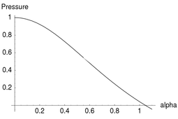
Figure 9: Pressure function P (α) with ρ 0 = 1, P c = 1 and Λ = 0

Page 28

Figure 10: Radius as a function of central pressure R = R(P c )

3.4 Solutions with positive cosmological constant

In the Schwarzschild-de Sitter spacetime there may exist a black-hole event horizon and there may also exist a cosmological event horizon. It depends on M and Λ in the Schwarzschild-de Sitter metric (2.22) which of the cases occur. The three possible cases were mentioned in the end of section 2.4.

3.4.1 Stellar models with spatially spherical geometry

0 < Λ < 4πρ 0

Integration of the TOV-Λ equation (3.1) leads to

Because of (3.30) the boundary P (R) = 0 exists. As in section 3.2.4 one finds

and written in terms of M , R and Λ again gives

Since the cosmological constant is positive the square root term is well defined if

Page 31

3.4.2 Solutions with exterior Nariai metric

Λ = 4πρ 0

In this special case integration of (3.1) gives

The pressure (3.45) vanishes at α = α b = π/2, the coordinate singularity in the radial coordinate r.

One would like to join the Schwarzschild-de Sitter metric. But with Λ = 4πρ 0 and M = (4π/3)ρ 0 R ³ it reads

The corresponding radius to α b is R = 3M . Therefore one would join both solutions at the horizon R = 3M . Since Λ = 4πρ 0 the radius R is also given √

by the cosmological constant R = 1/ 3M and the cosmological event horizon 1/ The interior metric reads

ds ² = −

The volume of group orbits of metric (3.46) is increasing whereas the group orbits of (3.47) have constant volume. Therefore it is not possible to join the vacuum solution (3.46) on as an exterior field to get the metric C ¹ at the P = 0 surface.

But there is the other spherically symmetric vacuum solution to the Einstein field equations with cosmological constant, the Nariai solution [15, 16], mentioned in chapter 2. Its metric is

ds ² =

where A and B are arbitrary constants. With r = e ^α this becomes

1 ds ² = . (3.49) Λ

Metrics (3.47) and (3.49) can be joined by fixing the constants A and B. With

Page 33

3.4.3 Solutions with decreasing group orbits at the boundary

4πρ 0 < Λ < Λ 0

Integration of (3.1) gives the pressure

Assume that the pressure vanishes before the second centre α = π of the 3-sphere is reached. The condition P (α = π) < 0 leads to an upper bound for the cosmological constant. This bound is given by

Then 4πρ 0 < Λ < Λ 0 implies the following:

The pressure is decreasing near the centre and vanishes for some α b , where π/2 < α b < π. Equations (3.4) and (3.6) imply that the volume of group orbits is decreasing if α > π/2.

At α b one uniquely joins the Schwarzschild-de Sitter solution by M = (4π/3)ρ 0 R ³ . With Gauss coordinates relative to the P (α b ) = 0 hypersurface the metric will be C ¹ . But there is a crucial difference to the former case with exterior Schwarzschild-de Sitter solution. Because of the decreasing group orbits at the boundary there is still the singularity r = 0 in the vacuum spacetime. Penrose-Carter diagram 32 shows this interesting solution. Figure 18 shows pressure (3.50). Figures 19 and 20 show the radius of the object as a function of the central pressure and the radius as a function of the new variable α, respectively. Constant density and central pressure are both set to one, ρ 0 = 1, P c = 1.

Page 35

3.4.4 Decreasing solutions with two regular centres

Λ 0 ≤ Λ < Λ E

As before the pressure is given by

Assume that the pressure is decreasing near the first centre α = 0. This gives an upper bound of the cosmological constant

Λ E := 4πρ 0 (3 P c /ρ 0 + 1) , (3.52)

where Λ E is the cosmological constant of the Einstein static universe. These possible values Λ 0 ≤ Λ < Λ E imply:

The pressure is decreasing is near the first centre α = 0 but remains positive for all α because Λ ≥ Λ 0 . Therefore there exists a second centre at α = π. At the second centre of the 3-sphere the pressure becomes

It only vanishes if Λ = Λ 0 . The solution is inextendible. The second centre is also regular. This is easily shown with Gauss coordinates. Recall metric (3.2) written in α

So one already used nearly Gauss coordinates up to a rescaling. With √ χ = α/ k this becomes

P c + ρ 0

ds ² = −

Thus the radius in terms of the Gauss coordinate is

√ 1 √ r(χ) = sin( kχ), (3.55) k

and both centres are regular because

Page 37

3.4.5 The Einstein static universe

Λ = Λ E

Assume a constant pressure function. Then the pressure gradient vanishes and therefore the right-hand side of (3.1) has to vanish. This gives an unique relation between density, central pressure and cosmological constant. One obtains (3.52)

Λ = Λ E = 4π (3P E + ρ 0 ) ,

where P E = P c was used to emphasise that the given central pressure corresponds to the Einstein static universe and is homogenous. Its metric is given by

ds ² = −dt ² + R E ,

where

R E is the radius of the three dimensional hyper-sphere t = const. The time component was rescaled to 1.

Thus for a given density ρ 0 there exists for every choice of a central pressure P c a unique cosmological constant given by (3.52) such that an Einstein static universe is the solution to (3.1). The constant pressure of the Einstein static universe is plotted in figure 23 with ρ 0 = 1 and P c = 1. Figure 24 shows the radius as a function of α. Solutions with two centres all have the same radial coordinate r = r(α).

Figure 24: Radial coordinate Figure 23: Pressure function P (α) r = r(α) with ρ 0 = 1, P c = 1 and Λ = 16π

Page 38

3.4.6 Increasing solutions with two regular centres

Λ E < Λ < Λ S

Integration of (3.1) again leads to

Assume that the pressure is finite at the second centre. This leads to an upper bound of the cosmological constant defined by

Λ S := 4πρ 0 (6 P c /ρ 0 + 4) . (3.58)

The possible values of the cosmological constant imply:

The pressure P (α) is increasing near the first regular centre. It increases monotonically up to α = π, where one has a second regular centre. This situation is similar to the case where Λ 0 ≤ Λ < Λ E . These solutions are also describing generalisations of the Einstein static universe. More can be concluded. The generalisations are symmetric with respect to the Einstein static universe. By symmetric one means the following. Instead of writing the pressure as a function of α depending on the given values ρ 0 , P c and Λ one can eliminate the cosmological constant with the pressure at the second centre P (α = π), given by (3.53). Let P c1 and P ^c2 denote the pressures of the first and second centre, respectively. Then the pressure can be written as

P (α)[P c1 , P c2 ] = ρ 0

This implies

π π P ( + α)[P c1 , P c2 ] = P ( − α)[P c2 , P c1 ]. (3.60) 2 2

Thus the pressure is symmetric to α = π/2 if both central pressures are exchanged and therefore this is the converse situation to the case where Λ 0 ≤ Λ < Λ E .

Another way of looking at it is to consider the pressure in terms of effective values, mentioned in section 2.3. Then the pressure reads

Page 40

3.4.7 Solutions with geometric singularity

Λ ≥ Λ S

In this case it is assumed that Λ exceeds the upper limit Λ S . Then (3.57) implies that the pressure is increasing near the centre and diverges before α = π is reached. In appendix B it is shown that the divergence of the pressure implies divergence of the squared Riemann tensor (B.3). Thus these solutions have a geometric singularity with unphysical properties. Therefore they are of no further interest. Figure 27 shows the divergent pressure.

Figure 27: Pressure function P (α) with ρ 0 = 1, P c = 1 and Λ = 50π

Page 42

4 Solutions with given equation of state

This chapter analyses the system of differential equations for a given monotonic equation of state. The choice of central pressure and central density together with the cosmological constant uniquely determines the pressure. The chapter is based on [18], where the following analysis was done without cosmological term. Geometrised units where c ² = 1/λ = 1 are used. The existence of a global solution for cosmological constants satisfying Λ < 4πρ b is shown, where ρ b denotes the boundary density. It turns out that solutions with negative cosmological constant are similar to those with vanishing cosmological constant. For positive cosmological constants new properties arise.

In section 4.1 Buchdahl variables are introduced. These new variables will help to proof the existence of global solutions and of stellar models. They are also helpful to derive analogous Buchdahl inequalities. Section 4.2 shows the existence of a regular solution at the centre. After remarks on extending the solution and a possible coordinate singularity the existence of global solutions is shown in section 4.5. For stellar models an analogous Buchdahl inequality is derived. Solutions without singularities are constructed. In particular for positive cosmological constants this is interesting because a second object has to be put in the spacetime to get a singularity free solution. The chapter ends with some remarks on finiteness of the radius.

4.1 Buchdahl variables

In chapter 2 metric function ν(r) was eliminated in (2.7) and (2.8) to give the TOV-Λ equation. Alternatively the pressure can be eliminated in the same equations. To do this Buchdahl [2] originally introduced the following variables:

It seems to be natural to do exactly the same, but using the new expression for e ^−a(r) which involves the cosmological constant. Alternatively it can be

Page 44

It is obvious that the terms with y ² ζ ² ,x drop out. Multiplying with ζ and using that

the following equation is obtained

Using again (4.7) one finds that

or rewritten using the product rule

The last two differential equations are identical to these obtained without a cosmological constant and as mentioned above, Λ is fully absorbed by the new variable y. The equation is linear in ζ and w. Derivation of (4.10) can also be done by rewriting the equation with vanishing cosmological constant in effective values for pressure and density. This leads to the Buchdahl variable y with w eff .

4.2 Existence of a unique regular solution at the centre

It is shown that there exists a unique regular solution in a neighbourhood of the centre r = 0 for each central density and given equation of state. To do this the following theorem is needed, see [18] for a proof.

Theorem 1 Let V be a finite dimensional real vector space, N : V → V a linear mapping, G : V × I → V a C ^∞ mapping and g : I → V a smooth mapping, where I is an open interval in R containing zero. Consider the equation

df s + N f = sG(s, f (s)) = g(s) (4.11) ds

for a function f defined on a neighbourhood of 0 and I and taking values in V . Suppose that each eigenvalue of N has a positive real part. Then there exists an open Interval J with 0 ∈ J ⊂ I and a unique bounded C ¹ function f on J \ 0 satisfying (4.11). Moreover f extends to a C ^∞ solution of (4.11) on J if N, G and g depend smoothly on a parameter z and the eigenvalues of N are distinct then the solution also depends smoothly on z.

Page 46

This disproves Collins [3] statement that for given equation of state, central pressure and cosmological constant the solution is not uniquely determined.

Standard theorems for differential equations imply that the solution can be extended as long as the right-hand sides of (2.16) or (4.13) are well defined. If the pressure satisfies P < ∞ and the denominator of (4.13) does not vanish, this means y = 1 − 2wx − (Λ/3)x > 0, then the right-hand sides are well defined. The second term involve the cosmological constant and therefore some new features will arise.

Uniqueness of the solution at the centre implies the following theorem.

Theorem 2 Suppose ρ(P ), P c and the cosmological constant Λ are given such that

note that (4π/3)ρ(P c ) = w c . Then the solution is the Einstein static universe with Λ E = Λ.

4.3 Extension of the solution

Theorem 3 Assume the pressure is decreasing near the centre, this means

Then the solution is extendible and the pressure is monotonically decreasing if

4πP + w − Λ/3 > 0. (4.19)

Proof. Suppose that ρ = ρ(P ), P c and Λ are given such that P is decreasing near the centre, then w(x) ,x ≤ 0. Using y > 0 because of the metric’s signature, (4.10) implies

(yζ ,x ) ,x ≤ 0. (4.20)

Rewriting (4.4) gives

Page 51

metric is at most C ¹ because the boundary density is larger than zero, this cannot be improved.

4.6 Generalised Buchdahl inequality

For stellar models an analogous Buchdahl inequality is derived. It turns out that the new inequality nearly coincides with the former (3.34), which was derived for constant density.

The proof of the following theorem solves the field equations with constant density written in Buchdahl variables. This solution is compared with a decreasing solution and leads to an analogous Buchdahl inequality. The solution with constant density is denoted with a tilde above.

Theorem 6 Let the cosmological constant be given such that Λ < 4πρ b . Then for stellar models there holds

1 Λ Λ 1 − 2w b r ² r ² b − b ≥ − . (4.36) 3 3 9w b

Proof. Assume that ρ(P ), P c and Λ are given such that the pressure is decreasing near the centre. In section 4.3 it was shown that this means that pressure and mean density are decreasing functions. Equation (4.10) implies

(˜ y ˜ ζ ,x ) ,x = 0 y ˜ ˜ ζ ,x = D, (4.37)

where D is a constant of integration.

If the density is constant ζ is the only unknown function in Einstein’s field equations.

The function ζ can be normalised to give ζ b = y b . The constant D is obtained from (4.4) evaluated at the boundary, therefore

1 Λ D = ˜ w − , (4.38) 2 6

which can be used to integrate (4.37). Notice that (4.7) reads

Λ −2˜ y ˜ y ,x = 2 ˜ w + . 3

The right-hand side of (4.37) can be written as